Microsoft Solver Foundation – Truck load optimization
Purpose: The purpose of this document is to illustrate how to use Microsoft Solver Foundation in order to resolve Truck load optimization problem.
Challenge: Truck load optimization problem is a typical problem in Distribution and Retail environments with Transportation management needs. For example, many companies have their own fleet or rent delivery trucks. In case you have a transportation load for a truck with packages of different sizes it may be so many ways you can load a truck. A natural question is "How do I load my truck in a best way?"
Solution: In this walkthrough we'll utilize the power of Microsoft Excel and Microsoft Solver Foundation in order to resolve Truck load optimization problem. Essentially our objective is to place as many packages into a truck as possible while satisfying a set constraints (2D/3D dimensions, total volume, etc.). In mathematics similar problem is known as "Squaring the square" (2D) or "Cubing the cube" (3D). Please find more info about Squaring the square problem here: http://en.wikipedia.org/wiki/Squaring_the_square
Schematically the solution may be presented in the following way (2D)

On this picture we have multiple packages of different sizes placed inside the rectangle (which may represent a truck). Obviously there's a number of ways you can load a truck and we'll be interested in one of feasible solutions which satisfies a set of logical constraints. At minimum we will need to make sure that our package is placed within defined truck area and there's no overlap of packages inside the truck
During the course of this walkthrough we'll build mathematical model to resolve the task using Microsoft Solver Foundation Add-in for Excel. And then upon resolution we'll visualize results using standard shapes in Excel. I also assume that the initial data set for analysis (Transportation loads) can be retrieved from Microsoft Dynamics AX 2012 using Web Services
Please note that for modeling using Microsoft Solver Foundation Add-in in Excel you will not need strong development skills. For mathematical modeling I'll be using very intuitive OML (Optimization Modeling Language). Please find detailed OML reference here: http://msdn.microsoft.com/en-us/library/ff524507(v=vs.93).aspx.
Walkthrough
Before we begin I will install Microsoft Solver Foundation Add-in for Excel

You can download it from Microsoft Solver Foundation product web site here: http://msdn.microsoft.com/en-us/devlabs/hh145003
Now let's start with formalization of the problem in Excel
First we'll address the problem of 2D Truck load optimization
Initial representation of the task

To even further simplify initial task we'll assume that we have to arrange squares (width = height). Thus in the matrix above TILE is a sequential square package number, SIDE is a width of square package, AREA is a calculated value of total area taken by square package, and finally X and Y define coordinates of where the package is placed inside a truck
On the picture below the matrix you can see how potential solution will look like with points (X, Y) defining coordinates of lower left corner of square package and SIDE defining package width and height
Now let's start building Microsoft Solver Foundation model
First off we'll introduce a set to represent TILE (square package)
Sets

Then we'll add a parameter for SIDE
Parameters

This info resides in Excel workbook, that's why we'll bind math model parameter SIDE to appropriate cells in Excel workbook
Binding Editor - SIDE

And this is how you specify Table/Range in Binding Editor. Please note how we define SIDEi: i = TILE and value field itself is SIDE
Excel workbook - SIDE

The next step is to define the decision. For this task our goal is to find X and Y coordinates of lower left corners of square packages and then we can place a package itself knowing its SIDE dimensions. That's why we can now define X[TILE] and Y[TILE] as below
Decisions - X

Similarly we can bind X[TILE] and Y[TILE] to Excel workbook cells which will display the results for us
Binding Editor - X

Please note that I still use the same selection for Table/Range. This time I just mapped Value field to X and Y columns correspondingly
Excel workbook – X
Decisions - Y

Binding Editor - Y

Excel workbook – Y
Please note that we don't define Goal because we are looking for one of feasible solutions which will satisfy a set of constraints. So to complete the model now we'll need to introduce appropriate constraints
Constraints - WITHINAREA

WITHINAREA constraint will help us to ensure that we place the package inside a truck
Expression - WITHINAREA
Foreach[{i,TILE},X[i]<=7-SIDE[i] & Y[i]<=7-SIDE[i]]
|
Constraints - NOOVERLAP

Now NOOVERLAP constraint will help us to ensure that packages inside the truck don't overlap which is logical
Expression - NOOVERLAP
Foreach[{i,9},{j,i+1,9}, X[i]>=X[j]+SIDE[j] | X[i]+SIDE[i]<=X[j] | Y[i]>=Y[j]+SIDE[j] | Y[i]+SIDE[i]<=Y[j] ]
|
Let's review the entire model now
Model

OML
Model[
Parameters[
Sets[Any],
TILE
],
Parameters[
Integers[0, Infinity],
SIDE[TILE]
],
Decisions[
Integers[0, Infinity],
X[TILE],
Y[TILE]
],
Constraints[
WITHINAREA -> Foreach[{i,TILE},X[i]<=7-SIDE[i] & Y[i]<=7-SIDE[i]],
NOOVERLAP -> Foreach[{i,9},{j,i+1,9}, X[i]>=X[j]+SIDE[j] | X[i]+SIDE[i]<=X[j] | Y[i]>=Y[j]+SIDE[j] | Y[i]+SIDE[i]<=Y[j] ]
]
]
|
Essentially this model is all you need to resolve a simplified Truck load optimization problem we initially formulated. And this is exactly what we are going to do right now
Log

Log
[11/18/2013 12:10:00 AM] Check started...
[11/18/2013 12:10:00 AM] Excel: 00:00:00.2699695
[11/18/2013 12:10:00 AM] Model syntax passed
[11/18/2013 12:10:00 AM] Model Check Complete
[11/18/2013 12:10:03 AM] Solve started...
[11/18/2013 12:10:04 AM] Excel: 00:00:00.0583775
[11/18/2013 12:10:04 AM] ===Solver Foundation Service Report===
Date: 11/18/2013 12:10:04 AM
Version: Microsoft Solver Foundation 3.0.2.10889 Express Edition
Model Name: DefaultModel
Capabilities Applied: CP
Solve Time (ms): 28
Total Time (ms): 142
Solve Completion Status: Feasible
Solver Selected: Microsoft.SolverFoundation.Solvers.ConstraintSystem
Algorithm: TreeSearch
Variable Selection: DomainOverWeightedDegree
Value Selection: ForwardOrder
Move Selection: Any
Backtrack Count: 24
===Solution Details===
Goals:
[11/18/2013 12:10:04 AM] Solve Complete
|
When you solve the model you will see the outcome as shown above
Please note that the system provides the solution and details of the algorithm which has been chosen to resolve the task. On the Solver Foundation Results tab you can now see values of X[TILE] and Y[TILE] corresponding to a feasible solution found
Result

Now we can also represent the optimal route visually using simple Excel graph
Excel workbook
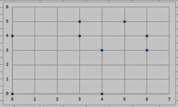
For example, this is how we can represent Tile 0 (0;0) which has SIDE = 4

Eventually we'll have the following packages layout in 2D

We've resolve a simplified task and now it is time to reformulate the problem to resolve a real-world 3D model with packages of different sizes (width, height, depth) and volumes. For visualization of the result after we solve 3D model we'll be using standard Excel shapes. You can find more info about how to programmatically use standard Excel shapes here: http://msdn.microsoft.com/en-us/library/office/ff744336.aspx
We'll start over with initial representation of the task for 3D model
Initial representation of the task

As you can see PACKAGE is a sequential number of package, WIDTH, DEPTH and HEIGHT are physical dimensions of a package, VOLUME represents package volume and X, Y and Z represent coordinates of a package in 3 dimensional truck space
We'll start with definition of set for PACKAGE
Sets - PACKAGE

This time we'll have 3 parameters representing WIDTH, DEPTH and HEIGHT as shown below
Parameters - WIDTH

Biding Editor - WIDTH

Parameters - DEPTH

Binding Editor - DEPTH

Parameters - HEIGHT

Binding Editor - HEIGHT

As you can see I mapped WIDTH, DEPTH and HEIGHT parameters to appropriate columns of the same matrix
Excel Workbook

Similarly I'll define a decision points representing package 3-dimensional coordinates X[PACKAGE], Y[PACKAGE] and Z[PACKAGE]
Decisions - X

Binding Editor - X

Decisions - Y

Binding Editor - Y

Decisions - Z

Binding Editor - Z

X, Y and Z coordinates will also be mapped against the same matrix as shown below
Excel Workbook
Still no defined Goals as we'll looking for one of feasible solutions for this task
And finally we'll define constraints similar to 2D case but this time taking into account all 3 coordinates (X, Y and Z)
Constraints - WITHINAREA

Expression - WITHINAREA
Foreach[{i,PACKAGE},X[i]<=5-WIDTH[i] & Y[i]<=12-DEPTH[i] & Z[i]<=2-HEIGHT[i]]
|
Constraints - NOOVERLAP

Expression - NOOVERLAP
Foreach[{i,5},{j,i+1,5}, X[i]>=X[j]+WIDTH[j] | X[i]+WIDTH[i]<=X[j] | Y[i]>=Y[j]+DEPTH[j] | Y[i]+DEPTH[i]<=Y[j] | Z[i]>=Z[j]+HEIGHT[j] | Z[i]+HEIGHT[i]<=Z[j]]
|
At this point we can review complete model
Model

OML
Model[
Parameters[
Sets[Any],
PACKAGE
],
Parameters[
Integers[0, Infinity],
WIDTH[PACKAGE],
DEPTH[PACKAGE],
HEIGHT[PACKAGE]
],
Decisions[
Integers[0, Infinity],
X[PACKAGE],
Y[PACKAGE],
Z[PACKAGE]
],
Constraints[
WITHINAREA -> Foreach[{i,PACKAGE},X[i]<=5-WIDTH[i] & Y[i]<=12-DEPTH[i] & Z[i]<=2-HEIGHT[i]],
NOOVERLAP -> Foreach[{i,5},{j,i+1,5}, X[i]>=X[j]+WIDTH[j] | X[i]+WIDTH[i]<=X[j] | Y[i]>=Y[j]+DEPTH[j] | Y[i]+DEPTH[i]<=Y[j] | Z[i]>=Z[j]+HEIGHT[j] | Z[i]+HEIGHT[i]<=Z[j]]
]
]
|
Next step is to run the model and review the result
Log

Log
[3/2/2014 3:44:34 PM] Solve started...
[3/2/2014 3:44:35 PM] Excel: 00:00:00.2532957
[3/2/2014 3:44:35 PM] ===Solver Foundation Service Report===
Date: 3/2/2014 3:44:35 PM
Version: Microsoft Solver Foundation 3.0.2.10889 Express Edition
Model Name: DefaultModel
Capabilities Applied: CP
Solve Time (ms): 54
Total Time (ms): 244
Solve Completion Status: Feasible
Solver Selected: Microsoft.SolverFoundation.Solvers.ConstraintSystem
Algorithm: TreeSearch
Variable Selection: DomainOverWeightedDegree
Value Selection: ForwardOrder
Move Selection: Any
Backtrack Count: 187
===Solution Details===
Goals:
[3/2/2014 3:44:35 PM] Solve Complete
|
The system successfully found a feasible solution for 3D Truck load optimization task and presented the results as shown below
Result

Now as we've got the results it would be nice to visualize them in a meaningful way
In order to do that with minimum effort I'm going to use VB.NET to programmatically render 3D Truck load in Excel using standard shapes (specifically cube(s))
Let's get going with VB.NET Macro now
VB.NET

I'll call my Macro GenerateData
Macro

Below I'll provide an example of how to visualize a sample Truck load optimization results
Microsoft Visual Basic for Applications

In the code below I use msoShapeCube to visually render Truck load in Excel. Please note that the idea here is to represent each package with a collection of building blocks – cubes, I also use the same color for building blocks of the same package for consistency
Below I provide a number of implementations of visualization moving from the very simple one to more and more sophisticated when I add groupings, introduce colors and more
Source code (1)
Sub GenerateData()
Set myDocument = Worksheets(1)
With myDocument.Shapes
.AddShape(msoShapeCube, 150, 150, 100, 100).Name = "shp11"
.AddShape(msoShapeCube, 225, 150, 100, 100).Name = "shp12"
.AddShape(msoShapeCube, 300, 150, 100, 100).Name = "shp13"
.AddShape(msoShapeCube, 375, 150, 100, 100).Name = "shp14"
.AddShape(msoShapeCube, 125, 175, 100, 100).Name = "shp21"
.AddShape(msoShapeCube, 200, 175, 100, 100).Name = "shp22"
.AddShape(msoShapeCube, 275, 175, 100, 100).Name = "shp23"
.AddShape(msoShapeCube, 350, 175, 100, 100).Name = "shp24"
.AddShape(msoShapeCube, 100, 200, 100, 100).Name = "shp31"
.AddShape(msoShapeCube, 175, 200, 100, 100).Name = "shp32"
.AddShape(msoShapeCube, 250, 200, 100, 100).Name = "shp33"
.AddShape(msoShapeCube, 325, 200, 100, 100).Name = "shp34"
.Range(Array("shp11", "shp12", "shp13", "shp14", "shp21", "shp22", "shp23", "shp24", "shp31", "shp32", "shp33", "shp34")).Group
End With
End Sub
|
Source code (2)
Sub GenerateData()
Set myDocument = Worksheets(1)
With myDocument.Shapes
.AddShape(msoShapeCube, 150, 150, 100, 100).Name = "shp111"
.AddShape(msoShapeCube, 225, 150, 100, 100).Name = "shp112"
.AddShape(msoShapeCube, 300, 150, 100, 100).Name = "shp113"
.AddShape(msoShapeCube, 375, 150, 100, 100).Name = "shp114"
.AddShape(msoShapeCube, 125, 175, 100, 100).Name = "shp121"
.AddShape(msoShapeCube, 200, 175, 100, 100).Name = "shp122"
.AddShape(msoShapeCube, 275, 175, 100, 100).Name = "shp123"
.AddShape(msoShapeCube, 350, 175, 100, 100).Name = "shp124"
.AddShape(msoShapeCube, 100, 200, 100, 100).Name = "shp131"
.AddShape(msoShapeCube, 175, 200, 100, 100).Name = "shp132"
.AddShape(msoShapeCube, 250, 200, 100, 100).Name = "shp133"
.AddShape(msoShapeCube, 325, 200, 100, 100).Name = "shp134"
.AddShape(msoShapeCube, 150, 75, 100, 100).Name = "shp211"
.AddShape(msoShapeCube, 225, 75, 100, 100).Name = "shp212"
.AddShape(msoShapeCube, 125, 100, 100, 100).Name = "shp221"
.AddShape(msoShapeCube, 200, 100, 100, 100).Name = "shp222"
.Range(Array("shp111", "shp112", "shp113", "shp114", "shp121", "shp122", "shp123", "shp124", "shp131", "shp132", "shp133", "shp134", "shp211", "shp212", "shp221", "shp222")).Group
End With
End Sub
|
Source code (3)
Sub GenerateData()
Set myDocument = Worksheets(1)
With myDocument.Shapes
Set shp111 = .AddShape(msoShapeCube, 150, 150, 100, 100)
shp111.Name = "shp111"
shp111.Fill.ForeColor.RGB = vbGreen
Set shp112 = .AddShape(msoShapeCube, 225, 150, 100, 100)
shp112.Name = "shp112"
shp112.Fill.ForeColor.RGB = vbGreen
Set shp113 = .AddShape(msoShapeCube, 300, 150, 100, 100)
shp113.Name = "shp113"
shp113.Fill.ForeColor.RGB = vbGreen
Set shp114 = .AddShape(msoShapeCube, 375, 150, 100, 100)
shp114.Name = "shp114"
shp114.Fill.ForeColor.RGB = vbGreen
Set shp121 = .AddShape(msoShapeCube, 125, 175, 100, 100)
shp121.Name = "shp121"
shp121.Fill.ForeColor.RGB = vbGreen
Set shp122 = .AddShape(msoShapeCube, 200, 175, 100, 100)
shp122.Name = "shp122"
shp122.Fill.ForeColor.RGB = vbGreen
Set shp123 = .AddShape(msoShapeCube, 275, 175, 100, 100)
shp123.Name = "shp123"
shp123.Fill.ForeColor.RGB = vbGreen
Set shp124 = .AddShape(msoShapeCube, 350, 175, 100, 100)
shp124.Name = "shp124"
shp124.Fill.ForeColor.RGB = vbGreen
Set shp131 = .AddShape(msoShapeCube, 100, 200, 100, 100)
shp131.Name = "shp131"
shp131.Fill.ForeColor.RGB = vbMagenta
Set shp132 = .AddShape(msoShapeCube, 175, 200, 100, 100)
shp132.Name = "shp132"
shp132.Fill.ForeColor.RGB = vbMagenta
Set shp133 = .AddShape(msoShapeCube, 250, 200, 100, 100)
shp133.Name = "shp133"
shp133.Fill.ForeColor.RGB = vbBlue
Set shp134 = .AddShape(msoShapeCube, 325, 200, 100, 100)
shp134.Name = "shp134"
shp134.Fill.ForeColor.RGB = vBlue
Set shp211 = .AddShape(msoShapeCube, 150, 75, 100, 100)
shp211.Name = "shp211"
shp211.Fill.ForeColor.RGB = vbRed
Set shp212 = .AddShape(msoShapeCube, 225, 75, 100, 100)
shp212.Name = "shp212"
shp212.Fill.ForeColor.RGB = vbRed
Set shp221 = .AddShape(msoShapeCube, 125, 100, 100, 100)
shp221.Name = "shp221"
shp221.Fill.ForeColor.RGB = vbRed
Set shp222 = .AddShape(msoShapeCube, 200, 100, 100, 100)
shp222.Name = "shp222"
shp222.Fill.ForeColor.RGB = vbRed
.Range(Array("shp111", "shp112", "shp113", "shp114", "shp121", "shp122", "shp123", "shp124", "shp131", "shp132", "shp133", "shp134", "shp211", "shp212", "shp221", "shp222")).Group
End With
End Sub
|
And here is the extract from the code above which highlights essential API methods used to implement this visualization
Sub GenerateData()
Set myDocument = Worksheets(1)
With myDocument.Shapes
Set shpGreen = .AddShape(msoShapeCube, 150, 150, 400, 100)
shpGreen.Name = "shpGreen"
shpGreen.Fill.ForeColor.RGB = vbGreen
Set shpMagenta = .AddShape(msoShapeCube, 100, 200, 200, 100)
shpMagenta.Name = "shpMagenta"
shpMagenta.Fill.ForeColor.RGB = vbMagenta
Set shpBlue = .AddShape(msoShapeCube, 250, 200, 200, 100)
shpBlue.Name = "shpBlue"
shpBlue.Fill.ForeColor.RGB = vbBlue
Set shpRed = .AddShape(msoShapeCube, 150, 75, 200, 100)
shpRed.Name = "shpRed"
shpRed.Fill.ForeColor.RGB = vbRed
.Range(Array("shpGreen", "shpMagenta", "shpBlue", "shpRed")).Group
End With
End Sub
|
When we implement visualization piece the next step is to embed this Macro into Excel Workbook
In order to save Excel workbook with VB.NET Macros you will have to Save Excel file as Excel Macro-Enabled Workbook

Now it is time to see the results of visualization in Excel
Here's how wire frame of Truck load would look like

And when we add colors and grouping here's how generated outcome will look like

Please note that I implemented 3D view in Excel by using simple standard Excel shapes (cube(s)) and I achieved 3D placement effect by working with 2D coordinates (X and Y) of those shapes
If necessary we can also add animation in Excel to dynamically play how Truck gets loaded with packages (in which sequence do they go into a truck, where do they go precisely inside a truck, etc.)
It may also make sense to introduce 2D projections of Truck body looking from different angles (side, top, bottom, etc.) for more detailed analysis
Result
<![if !supportLists]>- <![endif]>Complete 3D

<![if !supportLists]>- <![endif]>Step by Step 3D Animation
Step 1

Step 2

Step 3

Step 4
<![if !supportLists]>- <![endif]>6 x 2D Projections
Front

Side Left

Side Right

Back

Top

Bottom

In my future walkthroughs I plan to further address Truck load visualization problem by explaining how to develop Office App (HTML5/JavaScript) for Excel in order to deliver animation, rotation, drag-n-drop and other exciting interactive capabilities
Summary: In this document I illustrated how to use Microsoft Solver Foundation in order to resolve Truck load optimization problem. In particular in order to resolve this problem I used Microsoft Solver Foundation and Microsoft Excel providing robust platform for solving complex mathematical problems and rich visualization means to analyze the results of optimization. Please note that the data for initial analysis can be extracted from Microsoft Dynamics AX 2012 by means of Web Services. For visualization of results I used standard Excel shapes and developed VB.NET Macro to render Truck load optimization results straight inside Excel. It is important to mention that building models in Microsoft Solver Foundation Add-in for Excel doesn't require strong development skills, thus Business Analysts and Power Users may be very proficient in doing various optimizations using familiar Excel user interface. Please find more info about Modeling in Excel here: http://msdn.microsoft.com/en-us/library/ff524510(v=vs.93).aspx
Note: This document is intended for information purposes only, presented as it is with no warranties from the author. This document may be updated with more content to better outline the concepts and describe the examples.
Tags: Dynamics ERP, Dynamics AX 2012, Truck Load Optimization, Squaring the square, Cubing the cube, Solver Foundation, Excel, VB.NET, Macro, Web Services, Distribution, Retail, Transportation Management, Loads
Author: Alex Anikiev, PhD, MCP